Command-line utilities
grs-create
The most common algorithm to create a GRS is the LD pruning followed by p-value thresholding approach. This script provides a convenient implementation of this algorithm that can be easily integrated to computational pipelines.
This method consists of the following steps:
- Rank the variants by increasing p-value.
- Select the top variant, include it in the GRS and exclude all variants in LD
at a pre-defined threshold (
--ld-threshold). - Repeat 2. until the p-value threshold is reached (
--p-threshold).
Note
If a maf column is present in the summary statistics association file,
all variants that are too rare will be automaticall excluded when reading
the summary statistics file. If it is not available, the MAF will be
computed from the genotype data to allow filtering, which is more
computationally intensive.
For now, a plink binary file is required for the reference. A population-specific reference panel like the 1000 genomes phase 3 should be used.
This script generates a ‘grs’ file that is suitable for computing the GRS using grs-compute.
usage: grs-create [-h] [--p-threshold P_THRESHOLD] [--target-n TARGET_N]
                  [--maf-threshold MAF_THRESHOLD]
                  [--ld-threshold LD_THRESHOLD]
                  [--ld-window-size LD_WINDOW_SIZE] [--region REGION]
                  [--exclude-region EXCLUDE_REGION]
                  [--exclude-ambiguous-alleles] [--exclude-no-reference]
                  --summary SUMMARY --reference REFERENCE [--output OUTPUT]
                  [--debug]

optional arguments:
  -h, --help            show this help message and exit
  --p-threshold P_THRESHOLD
                        P-value threshold for inclusion in the GRS (default:
                        5e-8).
  --target-n TARGET_N   Target number of variants to include in the GRS.
  --maf-threshold MAF_THRESHOLD
                        Minimum MAF to allow inclusion in the GRS (default
                        0.05).
  --ld-threshold LD_THRESHOLD
                        LD threshold for the clumping step. All variants in LD
                        with variants in the GRS are excluded iteratively
                        (default 0.15).
  --ld-window-size LD_WINDOW_SIZE
                        Size of the LD window used to find correlated
                        variants. Making this window smaller will make the
                        execution faster but increases the chance of missing
                        correlated variants (default 1Mb).
  --region REGION       Only consider variants located WITHIN a genomic
                        region. The expected format is 'chrCHR:START-END'. For
                        example: 'chr1:12345-22345'.
  --exclude-region EXCLUDE_REGION
                        Only consider variants located OUTSIDE a genomic
                        region. The expected format is 'chrCHR:START-END'. For
                        example: 'chr1:12345-22345'.
  --exclude-ambiguous-alleles
                        Exclude variants with ambiguous alleles (e.g. G/C or
                        A/T)
  --exclude-no-reference
                        Exclude variants with no genotypes in the reference
                        panel.
  --summary SUMMARY     Path to the summary statistics files. Required columns
                        are 'name', 'chrom', 'pos', 'p-value', 'effect',
                        'reference' and 'risk'.
  --reference REFERENCE
                        Path the binary plink file containing reference
                        genotypes. These genotypes will be used for LD
                        clumping.
  --output OUTPUT, -o OUTPUT
                        Output prefix (default: grstools_selection).
  --debug
grs-compute
Computes the GRS using a ‘.grs’ file and individual-level genotypes.
The GRS are computed using the following formula:
Where \(GRS_i\) is the genetic risk score for the ith sample, j indexes the genetic variants included in the score, \(\beta_j\) is the coefficient estimated from the summary statistics and \(X_{ij}\) is the number of effect alleles carried by individual i at variant j.
Note
If the coefficient (\(\beta\)) is negative, it’s additive inverse is used instead (\(-\beta\)) and the effect and reference alleles are swapped accordingly. This ensures that contributions to the GRS are always positive.
Note
For missing genotypes, the mean dosage with respect to the effect allele is used when computing the variant’s contribution. Another intuitive way of handling this case would have been to set the contribution to 0, but doing so is a stronger claim than using the mean, especially for variants with a MAF close to 0.5.
If supported imputation data formats are used to hold the genotype information, the variants are further weighted by the INFO score as a form of global genotype confidence weighting:
Note
At this point, few data formats are supported. This is dependant on the use of the “ImputedVariant” class in the geneparse reader.
usage: grs-compute [-h] [--genotypes GENOTYPES]
                   [--genotypes-format GENOTYPES_FORMAT]
                   [--genotypes-kwargs GENOTYPES_KWARGS] --grs GRS [--out OUT]
                   [--ignore-genotype-quality] [--skip-strand-check]
                   [--exclude-strand-ambiguous] [--reference REFERENCE]
                   [--debug]

Compute the risk score.

optional arguments:
  -h, --help            show this help message and exit
  --genotypes GENOTYPES
                        File containing genotype data.
  --genotypes-format GENOTYPES_FORMAT
                        File format of the genotypes in the reference
                        (default: plink).
  --genotypes-kwargs GENOTYPES_KWARGS
                        Keyword arguments to pass to the genotypes container.
                        A string of the following format is expected:
                        'key1=value1,key2=value2,...It is also possible to
                        prefix the values by 'int:' or 'float:' to cast the
                        them before passing them to the constructor.
  --grs GRS             File describing the variants in the GRS. The expected
                        columns are 'name', 'beta', 'reference', 'risk'.
  --out OUT             Filename for the computed GRS (default:
                        computed_grs.csv).
  --ignore-genotype-quality
                        For imputed variants, if this flag is set, the
                        variants will not be weighted with respect to their
                        quality score. By default, the weights are used if
                        available.
  --skip-strand-check   Skips all the strand validation checks and assume that
                        the strand in the genotype and GRS files are the same.
                        This option should only be used if the variants were
                        manually curated. This option is also assumed if no
                        --reference is provided (with a warning).
  --exclude-strand-ambiguous
                        Exclude all strand ambiguous variants.
  --reference REFERENCE
                        Plink prefix for the reference genotypes. This is used
                        to find tags when needed or to compute the MAF.
  --debug
grs-mr
Mendelian randomization is a technique where genetic variants (or a genetic risk score (G)) is used to estimate the effect of an exposure (X) on an outcome (Y). Here, the estimation is done using the ratio method:
In the current implementation, bootstrap resampling is used to estimate the standard error which can be used for further inference.
usage: grs-mr [-h] [--grs-filename GRS_FILENAME] [--exposure EXPOSURE]
              [--outcome OUTCOME] [--exposure-type EXPOSURE_TYPE]
              [--outcome-type OUTCOME_TYPE]
              [--phenotypes-filename PHENOTYPES_FILENAME]
              [--phenotypes-sample-column PHENOTYPES_SAMPLE_COLUMN]
              [--phenotypes-separator PHENOTYPES_SEPARATOR]
              [--phenotype PHENOTYPE]

Estimate the effect of an exposure on an outcome using a GRS with an effect on
the exposure. Estimates are done using the ratio method.

optional arguments:
  -h, --help            show this help message and exit
  --grs-filename GRS_FILENAME
  --exposure EXPOSURE
  --outcome OUTCOME
  --exposure-type EXPOSURE_TYPE
                        Either continuous or discrete.
  --outcome-type OUTCOME_TYPE
                        Either continuous or discrete.
  --phenotypes-filename PHENOTYPES_FILENAME
  --phenotypes-sample-column PHENOTYPES_SAMPLE_COLUMN
  --phenotypes-separator PHENOTYPES_SEPARATOR
  --phenotype PHENOTYPE
grs-utils
This tool contains multiple features to manipulate GRS after they have been computed. Most of these tools either generate plots (as png files) or modified versions of the computed GRS. The latter file format is simply a CSV with a ‘sample’ and a ‘grs’ column.
histogram
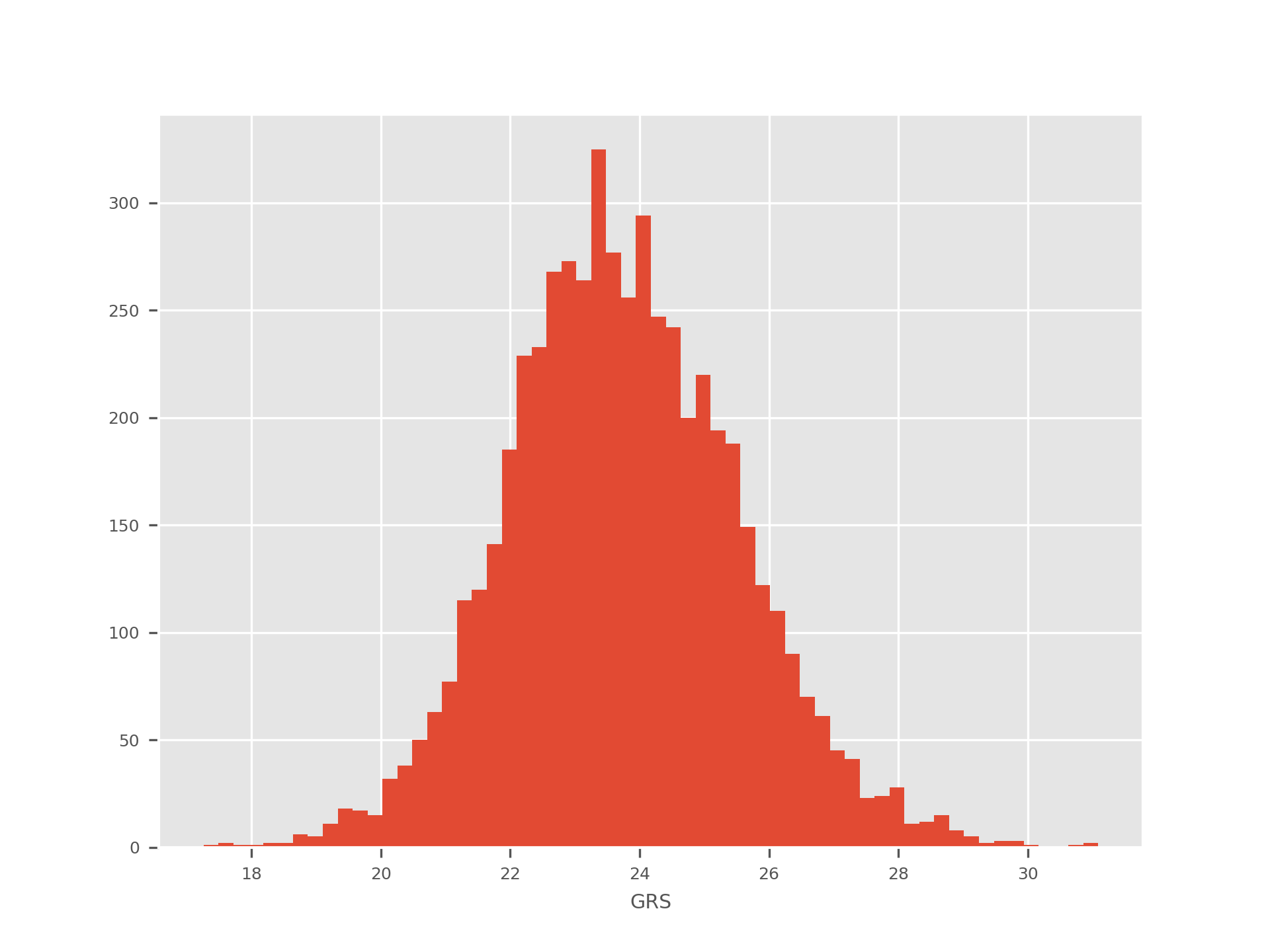
The histogram sub-command generates a histogram of all the GRS values. Here is an example:
quantiles
This function is used to dichotomize the GRS. The parameters are:
- -k The number of quantiles to take to form a group.
- -q The total number of quantiles.
Here are various examples of dichotomizations:
# Create two groups with respect to the median.
grs-utils quantiles my_grs.grs -k 1 -q 2

# 1st vs 5th quintiles.
grs-utils quantiles my_grs.grs -k 1 -q 5

# 1st vs 5th quintiles, but keeping all the samples (will be set to NA).
grs-utils quantiles my_grs.grs -k 1 -q 5 --keep-unclassified
The output file will contain two columns and a header: sample and
group. The group ‘0’ contains the individuals with lower values of the GRS
and the group ‘1’ contains individuals with high values of the GRS.
standardize
This function standardizes a GRS:
This function is useful when different GRS are to be compared. For example, is linear regression is used to assess the effect of a GRS on a given trait (Y), then the coefficient can be interpreted as the number of units increase in Y for a 1 s.d. increase in the GRS.
correlation
This utility takes two computed GRS files as input and plots the correlation between the GRS. This can be useful to test the variability of changing different hyperparameters (e.g. p-value threshold).
This script opens the plot in the interactive matplotlib viewer. From there, it can manipulated and saved to a file.
Here is an example:
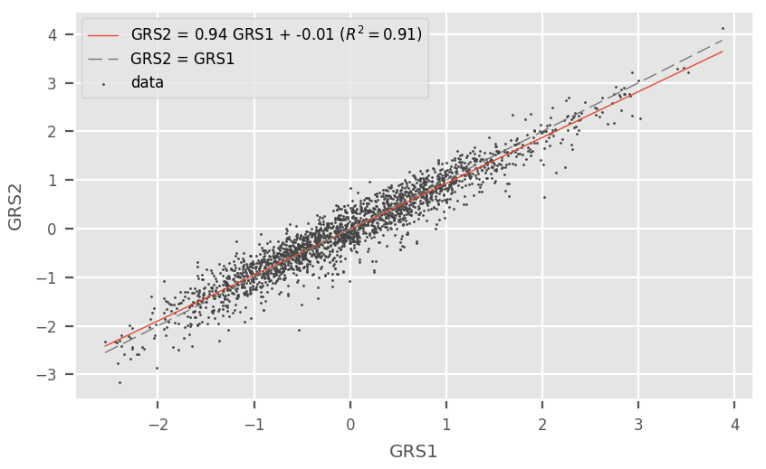
On the plot, the linear regression fit is displayed as well as the identity line to quickly assess the agreement between GRS.
usage: grs-utils [-h]
                 {histogram,quantiles,standardize,correlation,beta-plot,annotate-nearest-gene,locus-overlap}
                 ...

Utilities to manipulate computed GRS.

positional arguments:
  {histogram,quantiles,standardize,correlation,beta-plot,annotate-nearest-gene,locus-overlap}
    histogram           Plot the histogram of the computed GRS.
    quantiles           Dichotomize the GRS using quantiles. Takes two
                        parameters: k and q where q is the number of quantiles
                        and k is the cutoff to be used for the discretization.
                        For example, if the 1st quintile is to be compared to
                        the 5th, use -q 5 -k 1. By default -k=1 and -q=2 which
                        means the median is used.
    standardize         Standardize the GRS (grs <- (grs - mean) / std).
    correlation         Plot the correlation between two GRS.
    beta-plot           Compute beta coefficients from given genotypes data
                        and compare them with beta coefficients from the grs
                        file.
    annotate-nearest-gene
                        Annotate a GRS with the nearest gene for each SNP.
                        This script relies on an external gene annotation file
                        such as the GTF file provided by Ensembl.
    locus-overlap       Display variants in LD.

optional arguments:
  -h, --help            show this help message and exit
beta-plot
This utility compares the effect of variants between a summary statistics file in the GRS format and regression results using the user’s data. The goal is to ensure that the reported effect sizes are compatible and that there are no large or systematic discrepencies that could indicate a population or strand mismatch.
The utility also displays the standard errors on the plot. For the error of the expected coefficients, the standard errors are derived from the p-values and effect sizes.
Here is an example of the plot:
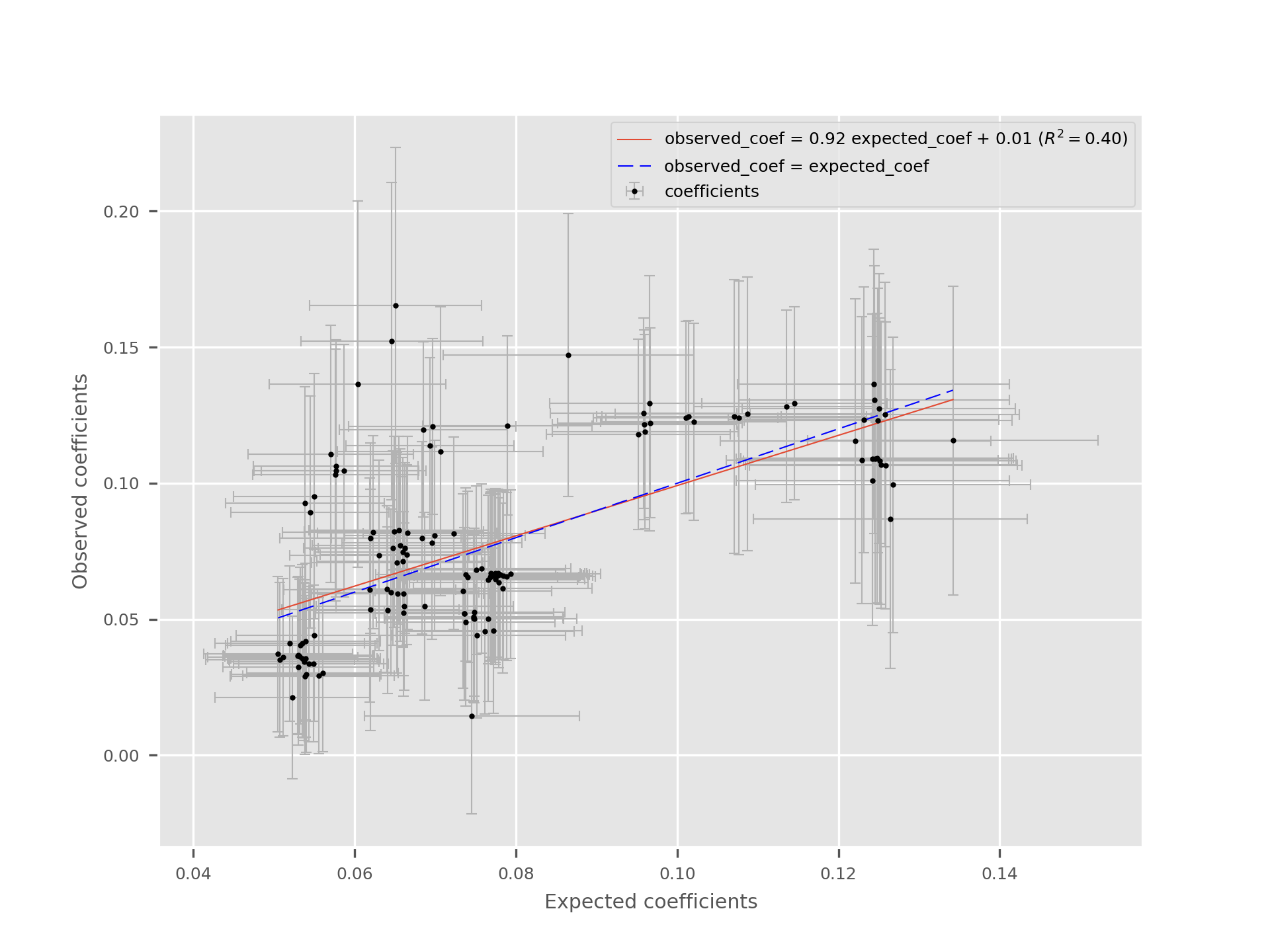
The execution also produces a text file displaying the SNPs information (chromosome, position, alleles, coefficients, standard errors, maf in the given population and n, the number of individuals used to compute each observed coefficient).
usage: grs-utils beta-plot [-h] --summary SUMMARY --genotypes-filename
                           GENOTYPES_FILENAME
                           [--genotypes-format GENOTYPES_FORMAT]
                           [--genotypes-kwargs GENOTYPES_KWARGS] --phenotype
                           PHENOTYPE --phenotypes-filename PHENOTYPES_FILENAME
                           [--phenotypes-separator PHENOTYPES_SEPARATOR]
                           [--phenotypes-sample-column PHENOTYPES_SAMPLE_COLUMN]
                           --test {linear,logistic} [--no-error-bars]
                           [--out OUT] [--svg] [--cpus CPUS] [--covar COVAR]

optional arguments:
  -h, --help            show this help message and exit
  --summary SUMMARY     File describing the selected variants for GRS. The
                        file must be in grs format
  --genotypes-filename GENOTYPES_FILENAME
                        File containing genotype data.
  --genotypes-format GENOTYPES_FORMAT
                        File format of the genotypes in the reference
                        (default:plink).
  --genotypes-kwargs GENOTYPES_KWARGS
                        Keyword arguments to pass to the genotype container.A
                        string of the following format is expected:
                        key1=value1,key2=value2...It is also possible to
                        prefix the values by 'int:' or 'float:' to cast them
                        before passing them to the constructor.
  --phenotype PHENOTYPE
                        Column name of phenotype in phenotypes file
  --phenotypes-filename PHENOTYPES_FILENAME
                        File containing phenotype data
  --phenotypes-separator PHENOTYPES_SEPARATOR
                        Separator in the phenotypes file (default:,).
  --phenotypes-sample-column PHENOTYPES_SAMPLE_COLUMN
                        Column name of target phenotype (default:sample).
  --test {linear,logistic}
                        Test to perform for beta coefficients estimation
  --no-error-bars       Do not show error bars on the plot
  --out OUT, -o OUT     Output name for beta coefficients plot and file
                        (default:observed_coefficients).
  --svg                 Use svg format for output plot (else will be .png)
  --cpus CPUS           Number of cpus to use for execution (default: number
                        of cpus - 1 = 7).
  --covar COVAR         Covariates other than the SNPs from summary stats.
                        Covariates should be in string form, separated by ,
                        covar1,covar2,covar3...
grs-evaluate
After calculating a GRS, it is important to quantify and evaluate its predictive performance. This tool provides multiple commands to easily run common diagnostics and validation steps.
regress
The regress subcommand assesses the effect of the GRS as a continuous trait on a given binary or continuous phenotype. In the case of a continuous outcome, linear regression is used and a plot like the following is generated:
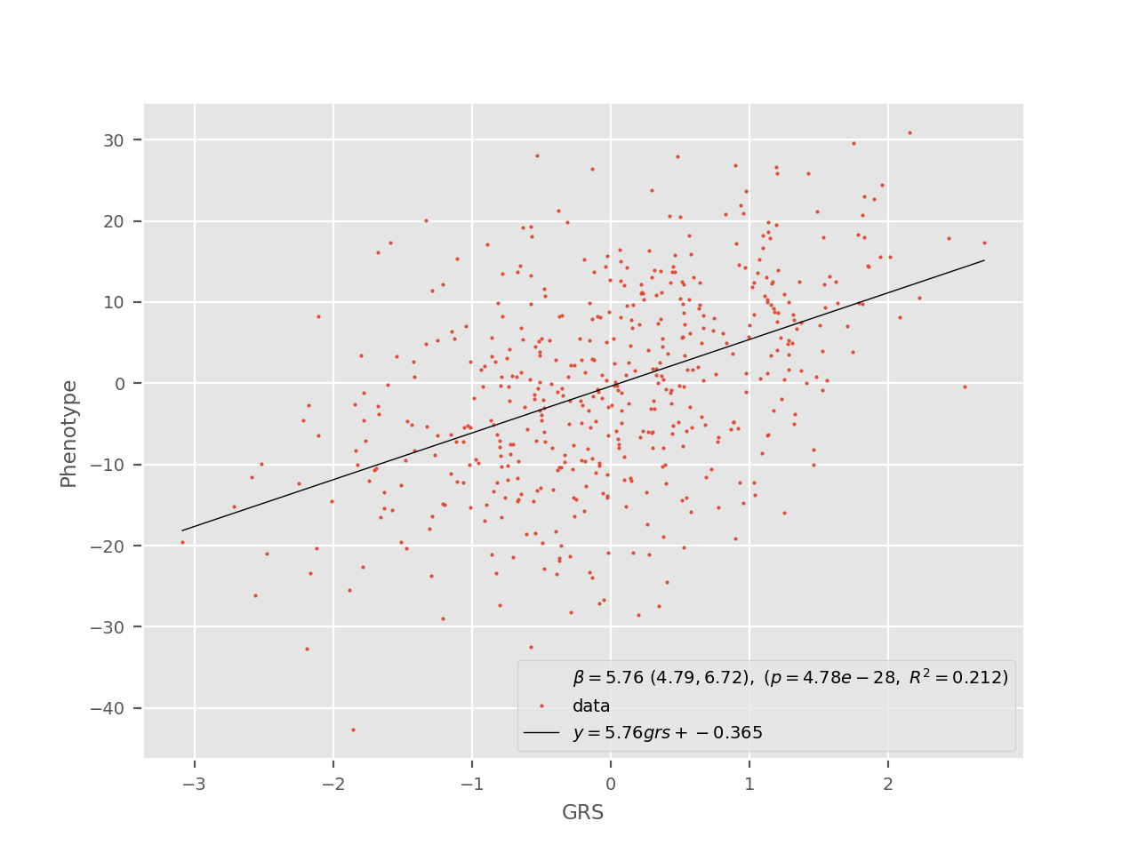
In this plot, it is possible to quickly validate that the GRS indeed has an effect on the trait of interest. It is also possible to estimate the fraction of the variance explained by the GRS (corresponding to the \(R^2\) value or to evaluate the expected change in the phenotype attributable to a 1 unit change in the GRS (\(\beta\) coefficient and its 95% CI). Note that standardizing the GRS first is useful to get an interpretation in units of GRS s.d. and to make comparisons across different GRS possible.
If the outcome is discrete, then logistic regression is better suited to evaluate the fit with the GRS. In this case, the generated plot looks as follows:
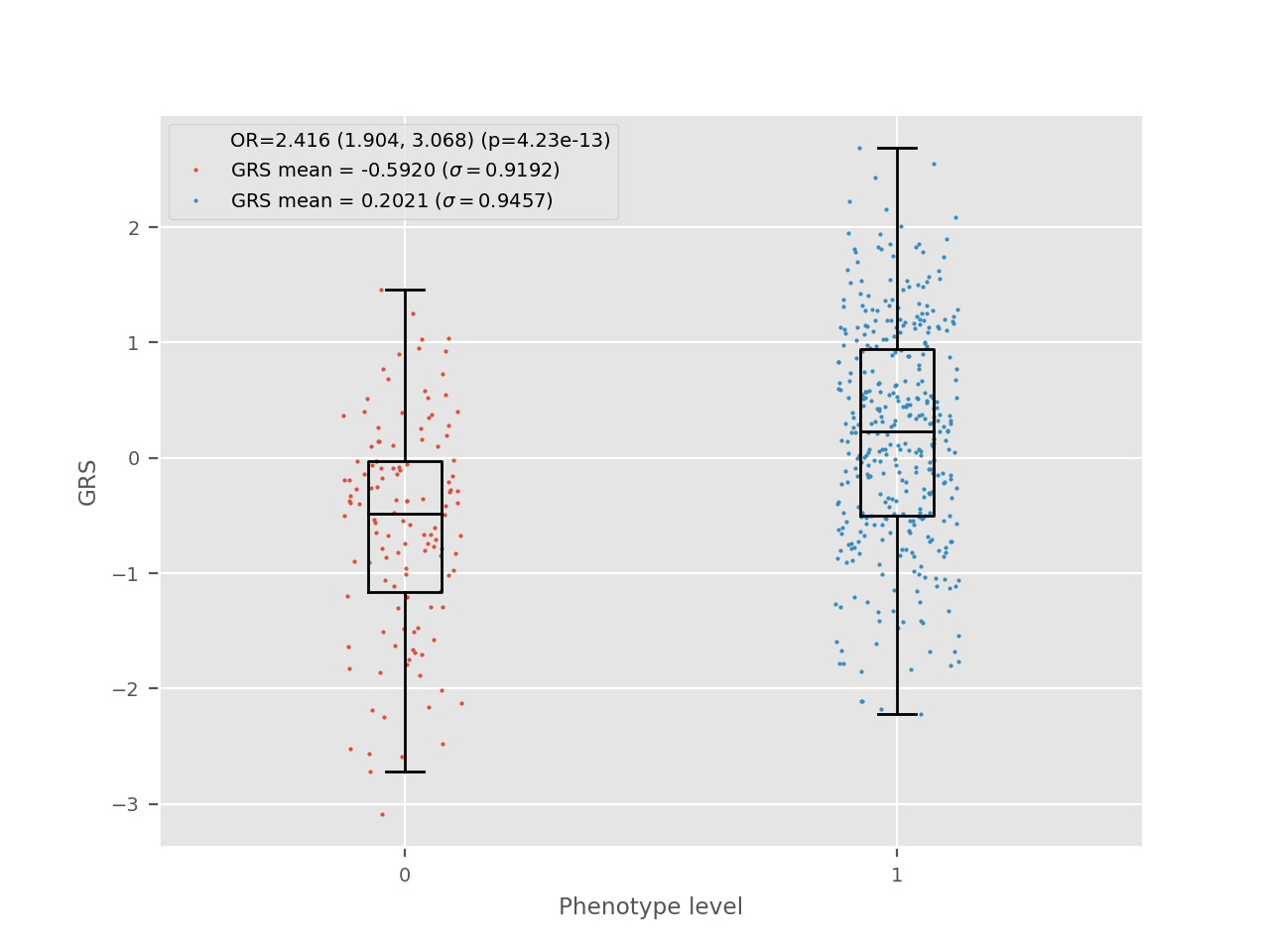
In this plot, the perspective is somewhat reversed, when compared with the linear case. The GRS is now in the y axis and its distribution is shown in cases and controls. The more general term “level” is used to describe the discrete numerical values of the phenotype as it could be used for factor variables.
The results for the logistic regression are shown on the plot. The OR corresponds to the expected increase in odds for a one unit increase in the GRS.
dichotomize-plot
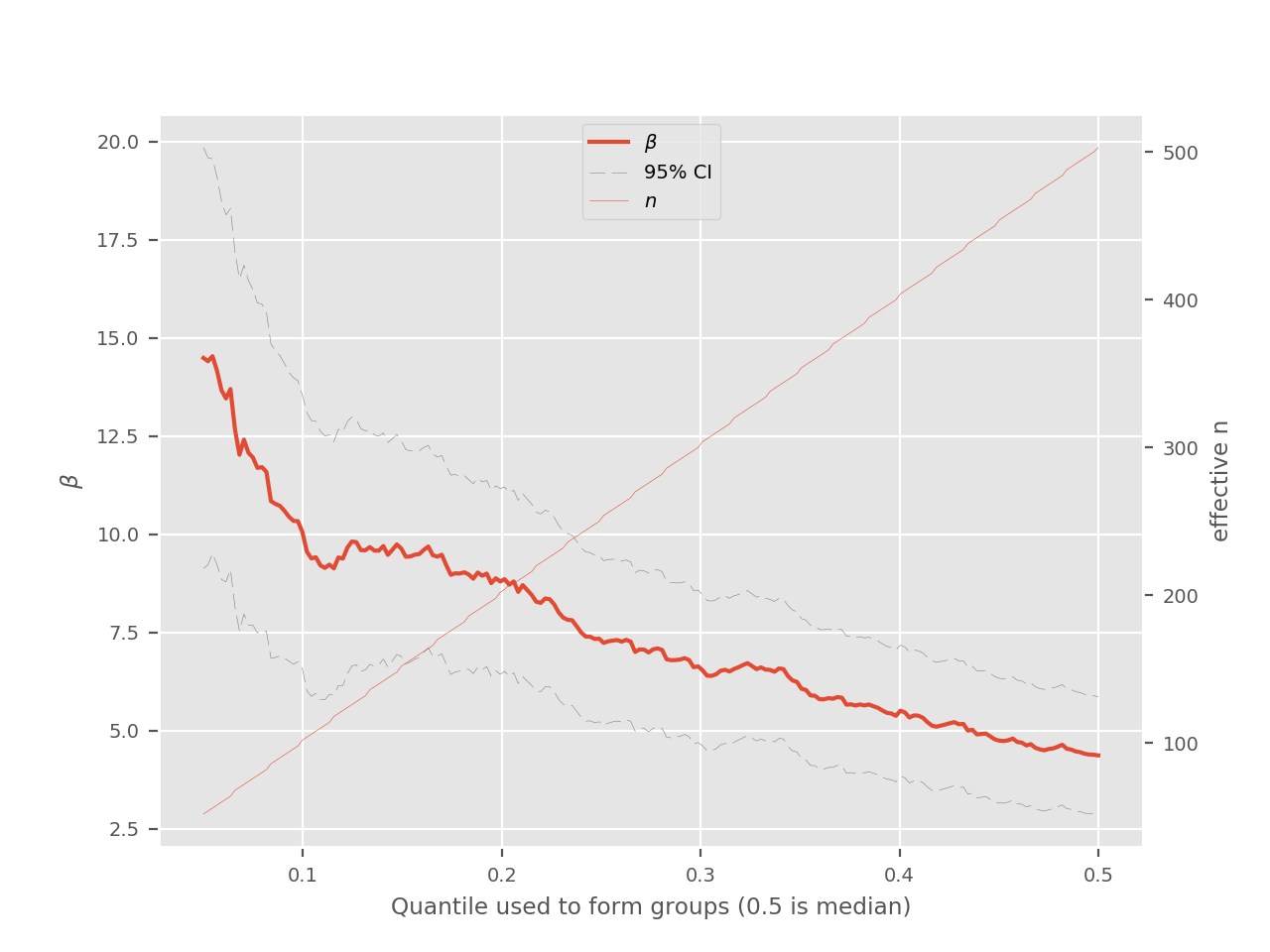
This plot can be used to select an optimal quantile for dichotmization. The tradeoff between the number of individuals classified and the GRS effect size is highlighted. Note that selecting a local maxima in this plot can be a bad idea because it increases the risk of overfitting. Traditional approaches such as using a test set, using cross-validation or bootstrapping can be used to select a more robust threshold.
The dichotmization is done by comparing the extremums of the distribution. For example, at the 0.25 quantile, the first quartile (1/4) is compared to the last quartile (4/4). All of the individuals in between can be used to form an “intermediate” group or can be excluded from downstream analyses. This is why the right axis represents the number of individuals that are classified in either the “high” or “low” group for a given dichotmization.
ROC
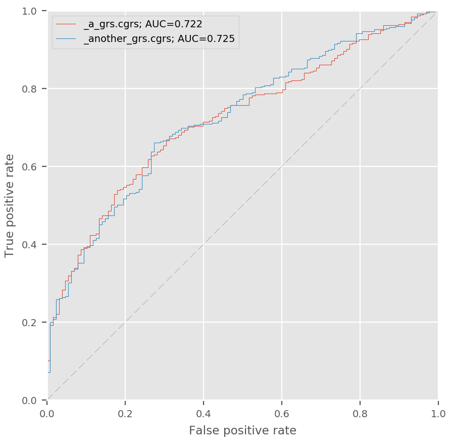
To evaluate the predictive accuracy of a GRS, it can be useful to look at its ROC curve.
usage: grs-evaluate [-h] {regress,dichotomize-plot,roc} ...

Utilities to evaluate the performance of GRS.

positional arguments:
  {regress,dichotomize-plot,roc}
    regress             Regress the GRS on a discrete or continuous outcome.
    dichotomize-plot    A plot to help identify ideal dichotmizatin
                        parameters.
    roc                 Draw a ROC curve for a GRS (given a binary phenotype).

optional arguments:
  -h, --help            show this help message and exit